Working with the metric
The metric is used extensively all around the package, both for bank generation and fitting factor computation.
All the relevant code is gathered in a single class mbank.metric.cbc_metric.
As shown in previous tutorials, to instantiate a metric, the user must specify:
The variable format: this defines the manifold the metric is defined on and sets the dimensionality of the space (see the help of
mbank.handlers.variable_handlerThe power spectral density (PSD): it characterizes the properties of the noise and affects the metric components
The frequency window for the analysis: the minimum and the maximum frequency for the analysis
The approximant: the name of a frequency domain
lalapproximant to compute the waveforms with
To instantiate the metric for a three dimensional manifold sampling over M, q, chi:
from mbank import cbc_metric
from mbank.utils import load_PSD
f, PSD = load_PSD('aligo_O3actual_H1.txt', True, 'H1')
metric = cbc_metric('Mq_chi',
			PSD = (f,PSD),
			approx = 'IMRPhenomD',
			f_min = 10, f_max = 1024)
The object has an internal frequency grid metric.f_grid, on which all the waveforms generated are evaluated as well as the PSD (stored in metric.PSD). The grid spacing is inferred from the given PSD whereas the limits are given by the frequency window.
To compute the metric at a given point, one can use the function get_metric(). Returning the metric evaluted at a given point theta. The function supports batch evaluation, as custom in numpy.
The argument metric_type allows the user to decide their preferred metric computation method. We strongly recommend to use the default method hessian, which computes the metric as the hessian of the overlap, as described in the paper: any other metric computation method either provides an experimental feature either shows a poor numerical performance!
A number of helpers allow to compute useful quantities derived from the metric:
get_metric_determinant: computes the determinant of the metricget_volume_element: computes the volume element of the space (the square root of the metric determinant)log_pdf: computes the logarithm of the volume element (useful for monte carlo sampling on the manifold)
The object also provides a method get_WF that returns the waveform evaluated a given value(s) of theta. It iteratively calls the lal function SimInspiralChooseFDWaveform through the helper method get_WF_lal.
To compute the match between two waveforms (evaluated on the standard frequency grid), the method match is available.
It can use the symphony match, extracting a random sky position and polarization.
If the overlap option is set to True, the time maximization implied by the match is not performed.
The function calls the underlying function get_WF_match which takes as an input the waveforms (rather than the manifold coordinates).
The following script compares the metric match with the actual match for two close values in the manifold:
heta1, theta2 = [20, 3, -0.8], [20.1,  3.05, -0.78]
metric.metric_match(theta1, theta2)
metric.match(theta1, theta2)
The metric can be computed starting from the gradients of the waveform. To compute the gradients you can call get_WF_grads which computes the gradients with a finite difference approximation. The user can control the order of the finite difference method as well as the step epsilon.
The gradients will be added on the last dimension of the returned array.
Below you can find an example:
theta = [[20, 3, -0.8], [10, 4, 0.4]]
WF = metric.get_WF(theta)
WF_grads = metric.get_WF_grads(theta)
Validating the metric
In many cases, it can be interesting to assess the accuracy of the metric as well as the numerical stabilty of its computation.
To ease this operation, we provide an executable mbank_validate_metric. The analysis is conduced on a given manifold at a given center. As usual, the options can be gathered in an ini file:
[validation]

variable-format: Mq_chi
center: 50 3.8 -0.6
psd: ./aligo_O3actual_H1.txt
asd: true
ifo: H1
approximant: IMRPhenomD

match: 0.97

f-min: 10
f-max: 1024
N-points: 500
epsilon: 1e-5
order: 4
metric-type: hessian
on-boundaries: false
overlap: false
show: true

save-dir: out_validation
Please, refer to mbank_validate_metric --help for more information on the arguments.
The command will produce several plots:
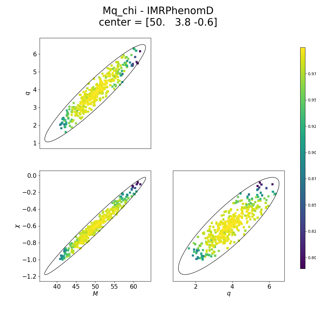
Constant match ellipses: given the center, an ellipse of constant match is plotted. A number of points (set by
N_points) is drawn inside (or, depending onon-boundaries, at the boundaries of) the ellipse. The true match of this points with the center is computed and it is reported on the colorbar
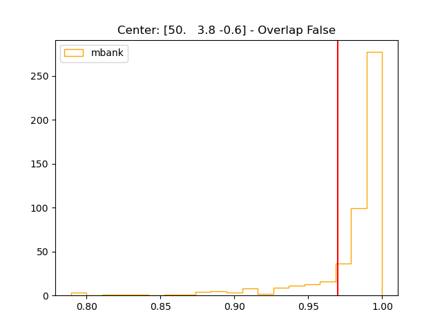
Match histogram: the distribution of matches computed for the
N_pointspoints is plotted on the histogram. A good metric approximation, will show very very few points below the red line, corresponding to the user defined match for the ellipses.
True match plot: for each of the eigendirection of the metric, the relation between match and distance from the center is computed and plotted. In green, it is plotted the same relation as predicted by the metric. The dashed lines report the results of a 2 and 4 dimensional fit.

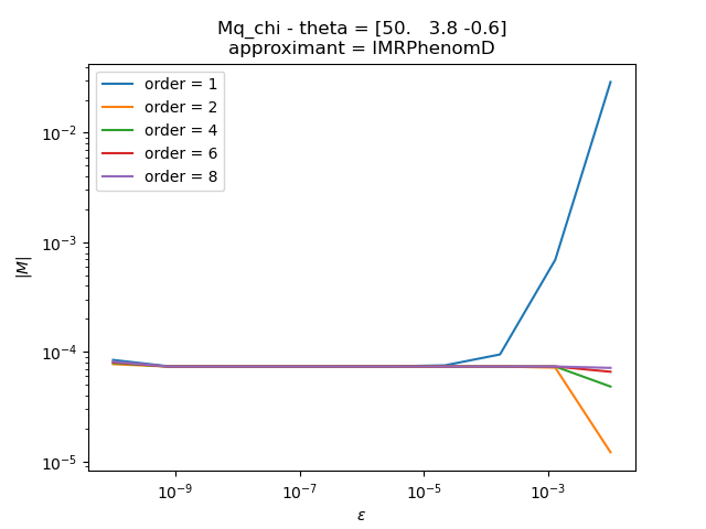
|M| stability: plot of the relation between the determinant of the metric and the step for the finite difference method, for different orders of the derivative.
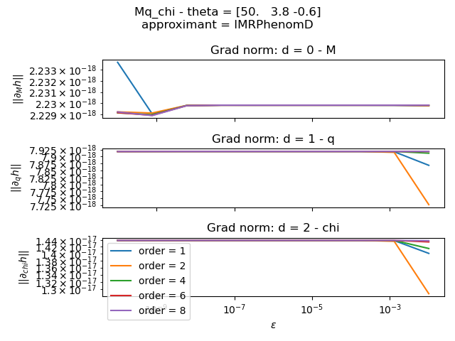
gradient stability: plot of the L2 norm of the gradients as a function of the step epsilon for the finite difference method. Again, each series refers to a different order