How to perform injections
The injection code throws injections in the bank and computes the match of each of them with the templates. The injections can be either loaded by file either randomly generated within each tile.
Many options are in common with mbank_place_templates. The options unique to the mbank_injections are:
bank-file: name of the bank fileinj-file: an xml file to load a generic set of injection from. It can be generated withmbank_injfile, which can draw injections from a given normalizing flow model.n-injs: how many injections to perform? They will randomly placed in the space so that each tile will keep a number of injections proportional to the volume.full-match: whether to compute the full match, rather than just the metric approximationmchirp-window: relative chirp mass window. For each injection, we compute the match only with the templates with a relative difference in chirp mass less thanmchirp-window.
Injections from command line
Assuming you generated the bank normally in the previous section, you can use the same ini file to generate the injection file and to perform the injection study.
By running
mbank_injfile my_first_eccentric_bank.ini
mbank_injections my_first_eccentric_bank.ini
This will produce two nice plots.
The histogram of the fitting factor of each injection (i.e. best match of an injection with the templates)

and a scatter plot with the injections with fitting factor smaller that mm:
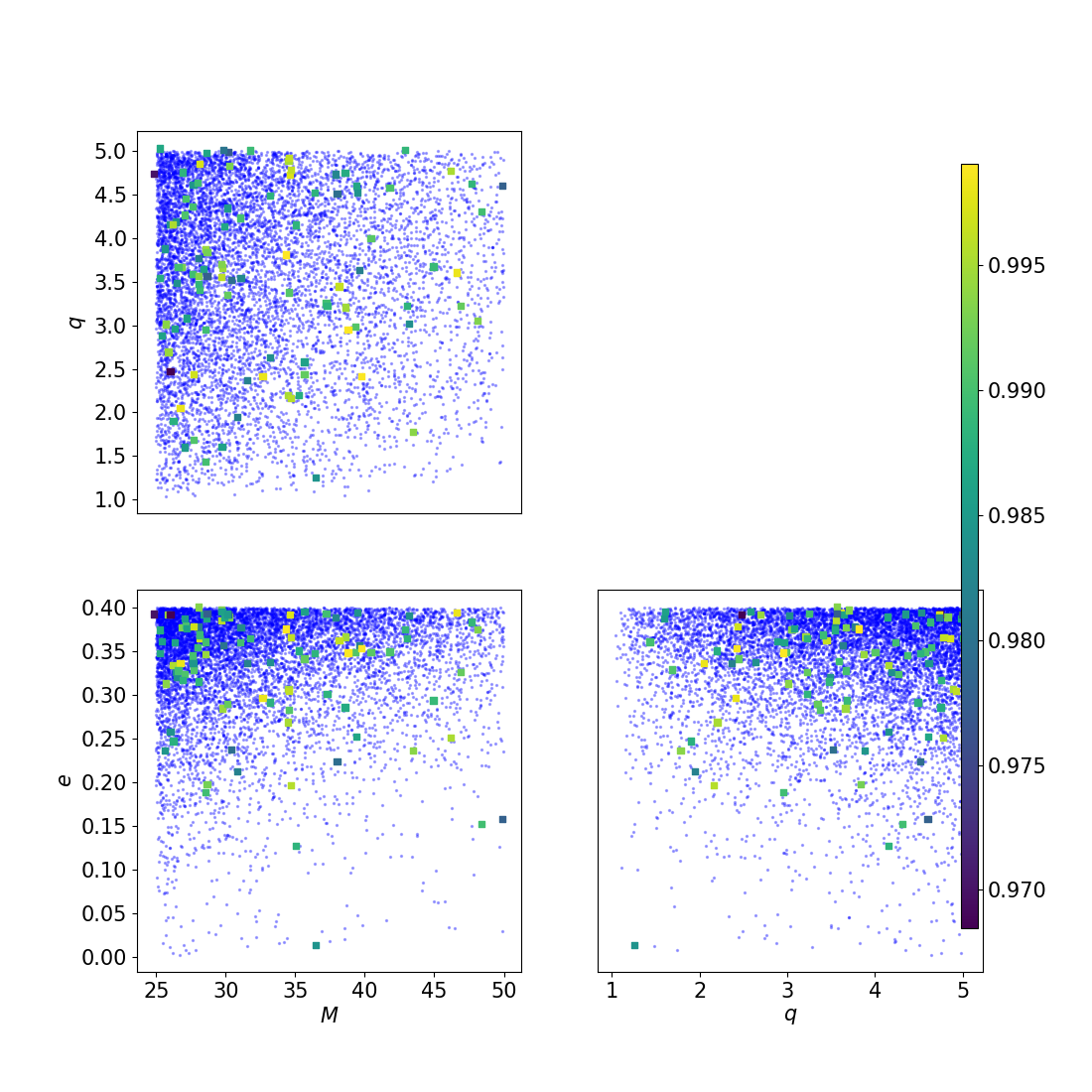
As you see very very few injections have fitting factor below 0.97, which means that the bank is doing a good job at covering the space.
Injections by hands
Again, we can also perform injections using a python script (although this is not advised).
Here we assume we have at hand a three dimensional bank bank.dat and a flow flow.zip, with the variable format Mq_chi: this was generated in the previous page.
After the imports,
from mbank import variable_handler, cbc_metric, cbc_bank
from mbank.utils import compute_injections_match, get_random_sky_loc, initialize_inj_stat_dict
from mbank.utils import load_PSD, plot_tiles_templates
from mbank.flow import STD_GW_Flow
import numpy as np
you need to load the bank and the flow and to instantiate a mbank.metric.cbc_metric object:
bank = cbc_bank('Mq_chi', 'bank.dat')
flow = STD_GW_Flow.load_flow('flow.zip')

metric = cbc_metric(bank.variable_format,
	PSD = load_PSD('aligo_O3actual_H1.txt', True, 'H1', df = 1),
	approx = 'IMRPhenomD',
	f_min = 10, f_max = 1024)
We then generate the injections by sampling them from the normalizing flow model:
n_injs = 100
injs_3D = flow.sample(n_injs)
injs_12D = bank.var_handler.get_BBH_components(injs_3D, bank.variable_format)
sky_locs = np.column_stack(get_random_sky_loc(n_injs))
stat_dict = initialize_inj_stat_dict(injs_12D, sky_locs = sky_locs)
In this case injections are sampled in the 3D space of \(M, q, \chi_{eff}\) but since injections can be generic, we need to cast them in the full 12 dimensional BBH space. We also draw at random the sky locations for the injections: setting it to None, will set \(F_\times = 0\).
In the last line, we initialized an “injection statistics dictionary”, which will store information about the fitting factor computations.
It’s now time to go ahead, be patient and perform the fitting factor computation:
inj_stat_dict = compute_injections_match(stat_dict, bank,
	metric_obj = metric, mchirp_window = 0.1, symphony_match = True)
save_inj_stat_dict('injections.json', inj_stat_dict)
This will take several minutes… You can then save the injection stat dictionary in json format and plot the result of the injection study.
plot_tiles_templates(bank.templates, bank.variable_format,
	injections = injs_3D, inj_cmap = stat_dict['match'], show = True)
Injections with condor
If you are on a cluster with HTCondor, it is very likely that you want to put the injection computation inside a condor DAG, to run in parallel. Luckily, mbank does also that for you. To set up the dag you just need to type:
mbank_injections_workflow --n-jobs 100 --inj-file eccentric_bank/eccentric_injections.xml my_first_eccentric_bank.ini
This will load the injections from the file eccentric_bank/eccentric_injections.xml and will split the computation between 100 jobs.
The command will produce many files, including a mbank_injections_dag.dag file, which keeps the instructions to run all the jobs in the DAG, and two submit files (match_computation.sub and merge_products.sub), which keeps the instructions to run the actual jobs.
Note that, depending on your local condor configuration, you may need to edit the submit files to make the DAG run smoothly.
Once you are ready, you can launch the DAG and monitor its advancment with
condor_submit_dag mbank_injections_dag.dag
tail -f mbank_injections_dag.dag.dagman.out
Once the DAG is over, you can find the json output file together with some plots in the directory results.
To clean all the temporary files you produced, you can run
mbank_injections_workflow --clean
Pay attention that this will erase also the result directory, so make sure to move it somewhere safe before clening everything.